TensorBoard: Visualizing Learning
(TensorBoard : 학습 시각화)
기계학습이 어떻게 하는지 시각적으로 볼 수 있는 라이브러리입니다.
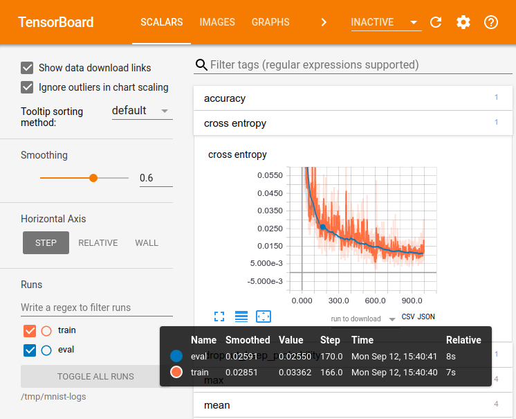
거대한 심 신경 네트워크를 훈련하는 것처럼 TensorFlow를 사용할 계산은 복잡하고 혼란 스러울 수 있습니다. TensorFlow 프로그램을 더 쉽게 이해하고 디버깅하고 최적화하기 위해 TensorBoard라는 시각화 도구 모음을 포함 시켰습니다. TensorBoard를 사용하여 TensorFlow 그래프를 시각화하고 그래프 실행에 대한 정량적 메트릭을 플롯하고 통과 한 이미지와 같은 추가 데이터를 표시 할 수 있습니다. TensorBoard가 완전히 구성되면 다음과 같이 표시됩니다.
이 자습서는 간단한 TensorBoard 사용법을 배우기위한 것입니다. 다른 리소스도 있습니다. TensorBoard의 GitHub(TensorBoard's GitHub)에는 팁 및 트릭 및 디버깅 정보를
포함하여 TensorBoard 사용에 대한 더 많은 정보가 있습니다.
Serializing the data
데이터 직렬화
TensorBoard는 TensorFlow를 실행할 때 생성 할 수있는 요약 데이터가 포함 된 TensorFlow 이벤트 파일을 읽음으로써 작동합니다. 다음은 TensorBoard 내의 요약 데이터에 대한 일반적인 수명주기입니다.
먼저 요약 데이터를 수집 할 TensorFlow 그래프를 만들고 요약 작업으로 주석(summary operations)을 추가 할 노드를 결정합니다.
예를 들어, MNIST 자리를 인식 할 수있는 길쌈 신경 네트워크를 학습한다고 가정합니다. 학습 속도가 시간에 따라 어떻게 변하는 지, 그리고 목적 함수가 어떻게 변하는지를 기록하고 싶습니다. 학습 속도와 손실을 각각 출력하는 노드에 tf.summary.scalar op를 연결하여이를 수집합니다. 그런 다음 각 스칼라 요약에 '학습률'또는 '손실 함수'와 같은 의미있는 태그를 지정합니다.
특정 레이어에서 나오는 활성화 분포 또는 그라데이션이나 가중치의 분포를 시각화하고 싶을 수도 있습니다. tf.summary.histogram ops를 그라디언트 출력과 가중치를 유지하는 변수에 각각 첨부하여이 데이터를 수집합니다.
사용 가능한 모든 요약 작업에 대한 자세한 내용은 요약 작업에 대한 문서를 확인하십시오.
TensorFlow의 작업은 실행하기 전까지는 아무 것도하지 않거나 출력에 의존하는 연산을 수행합니다. 방금 작성한 요약 노드는 그래프의 주변 장치입니다. 현재 실행중인 작업 단위는 모두 해당 노드에 의존하지 않습니다. 따라서 요약을 생성하려면 이러한 모든 요약 노드를 실행해야합니다. 손으로 직접 관리하는 것은 지루할 수 있으므로 tf.summary.merge_all을 사용하여 모든 요약 데이터를 생성하는 단일 op로 결합하십시오.
그런 다음 병합 된 요약 연산을 실행하면 주어진 단계에서 모든 요약 데이터가있는 직렬화 된 요약 protobuf 객체가 생성됩니다. 마지막으로이 요약 데이터를 디스크에 기록하려면 summary protobuf를 tf.summary.FileWriter에 전달하십시오.
FileWriter는 생성자에서 logdir을 사용합니다.이 logdir은 모든 이벤트가 기록되는 디렉토리입니다. 또한 FileWriter는 선택적으로 생성자에서 Graph를 가져올 수 있습니다. Graph 객체를 받으면 TensorBoard는 텐서 모양 정보와 함께 그래프를 시각화합니다. 이렇게하면 그래프를 통해 흐르는 것이 훨씬 잘 전달됩니다 : Tensor 모양 정보( Tensor shape information)를 참조하십시오.
이제 그래프를 수정하고 FileWriter를 만들었으므로 네트워크를 시작할 준비가되었습니다! 원하는 경우 매 단계마다 병합 된 요약 작업을 실행하고 많은 양의 교육 데이터를 기록 할 수 있습니다. 그것은 당신이 필요로하는 것보다 더 많은 데이터 일 것 같다. 대신 병합 된 요약 연산을 n 단계마다 실행하는 것을 고려하십시오.
아래의 코드 예제는 간단한 MNIST 튜토리얼을 수정 한 것으로서 몇 가지 요약 작업을 추가하고 10 단계마다 실행합니다. 이것을 실행하고 tensorboard --logdir = / tmp / tensorflow / mnist를 실행하면 훈련 도중 가중치 나 정확도가 어떻게 변화했는지와 같은 통계를 시각화 할 수 있습니다. 아래의 코드는 발췌 한 것입니다. 전체 소스가 여기(here)에 있습니다.
def variable_summaries(var):
  """Attach a lot of summaries to a Tensor (for TensorBoard visualization)."""
  with tf.name_scope('summaries'):
    mean = tf.reduce_mean(var)
    tf.summary.scalar('mean', mean)
    with tf.name_scope('stddev'):
      stddev = tf.sqrt(tf.reduce_mean(tf.square(var - mean)))
    tf.summary.scalar('stddev', stddev)
    tf.summary.scalar('max', tf.reduce_max(var))
    tf.summary.scalar('min', tf.reduce_min(var))
    tf.summary.histogram('histogram', var)

def nn_layer(input_tensor, input_dim, output_dim, layer_name, act=tf.nn.relu):
  """Reusable code for making a simple neural net layer.

  It does a matrix multiply, bias add, and then uses relu to nonlinearize.
  It also sets up name scoping so that the resultant graph is easy to read,
  and adds a number of summary ops.
  """
  # Adding a name scope ensures logical grouping of the layers in the graph.
  with tf.name_scope(layer_name):
    # This Variable will hold the state of the weights for the layer
    with tf.name_scope('weights'):
      weights = weight_variable([input_dim, output_dim])
      variable_summaries(weights)
    with tf.name_scope('biases'):
      biases = bias_variable([output_dim])
      variable_summaries(biases)
    with tf.name_scope('Wx_plus_b'):
      preactivate = tf.matmul(input_tensor, weights) + biases
      tf.summary.histogram('pre_activations', preactivate)
    activations = act(preactivate, name='activation')
    tf.summary.histogram('activations', activations)
    return activations

hidden1 = nn_layer(x, 784, 500, 'layer1')

with tf.name_scope('dropout'):
  keep_prob = tf.placeholder(tf.float32)
  tf.summary.scalar('dropout_keep_probability', keep_prob)
  dropped = tf.nn.dropout(hidden1, keep_prob)

# Do not apply softmax activation yet, see below.
y = nn_layer(dropped, 500, 10, 'layer2', act=tf.identity)

with tf.name_scope('cross_entropy'):
  # The raw formulation of cross-entropy,
  #
  # tf.reduce_mean(-tf.reduce_sum(y_ * tf.log(tf.softmax(y)),
  #                               reduction_indices=[1]))
  #
  # can be numerically unstable.
  #
  # So here we use tf.nn.softmax_cross_entropy_with_logits on the
  # raw outputs of the nn_layer above, and then average across
  # the batch.
  diff = tf.nn.softmax_cross_entropy_with_logits(targets=y_, logits=y)
  with tf.name_scope('total'):
    cross_entropy = tf.reduce_mean(diff)
tf.summary.scalar('cross_entropy', cross_entropy)

with tf.name_scope('train'):
  train_step = tf.train.AdamOptimizer(FLAGS.learning_rate).minimize(
      cross_entropy)

with tf.name_scope('accuracy'):
  with tf.name_scope('correct_prediction'):
    correct_prediction = tf.equal(tf.argmax(y, 1), tf.argmax(y_, 1))
  with tf.name_scope('accuracy'):
    accuracy = tf.reduce_mean(tf.cast(correct_prediction, tf.float32))
tf.summary.scalar('accuracy', accuracy)

# Merge all the summaries and write them out to /tmp/mnist_logs (by default)
merged = tf.summary.merge_all()
train_writer = tf.summary.FileWriter(FLAGS.summaries_dir + '/train',
                                      sess.graph)
test_writer = tf.summary.FileWriter(FLAGS.summaries_dir + '/test')
tf.global_variables_initializer().run()
FileWriter를 초기화 한 후에는 모델을 테스트하고 테스트 할 때 FileWriter에 요약을 추가해야합니다.
# Train the model, and also write summaries.
# Every 10th step, measure test-set accuracy, and write test summaries
# All other steps, run train_step on training data, & add training summaries

def feed_dict(train):
  """Make a TensorFlow feed_dict: maps data onto Tensor placeholders."""
  if train or FLAGS.fake_data:
    xs, ys = mnist.train.next_batch(100, fake_data=FLAGS.fake_data)
    k = FLAGS.dropout
  else:
    xs, ys = mnist.test.images, mnist.test.labels
    k = 1.0
  return {x: xs, y_: ys, keep_prob: k}

for i in range(FLAGS.max_steps):
  if i % 10 == 0:  # Record summaries and test-set accuracy
    summary, acc = sess.run([merged, accuracy], feed_dict=feed_dict(False))
    test_writer.add_summary(summary, i)
    print('Accuracy at step %s: %s' % (i, acc))
  else:  # Record train set summaries, and train
    summary, _ = sess.run([merged, train_step], feed_dict=feed_dict(True))
    train_writer.add_summary(summary, i)
이제 TensorBoard를 사용하여이 데이터를 시각화 할 수 있습니다.
Launching TensorBoard
TensorBoard 출시
TensorBoard를 실행하려면 다음 명령을 사용하십시오 (또는 python -m tensorboard.main).
tensorboard --logdir=path/to/log-directory여기서 logdir은 FileWriter가 데이터를 직렬화 한 디렉토리를 가리 킵니다. 이 logdir 디렉토리에 별도의 실행에서 직렬화 된 데이터가 들어있는 하위 디렉토리가 있으면 TensorBoard는 이러한 모든 실행에서 데이터를 시각화합니다. TensorBoard가 실행되면 웹 브라우저에서 localhost : 6006으로 이동하여 TensorBoard를 봅니다.
TensorBoard를 보면 오른쪽 상단 모서리에 탐색 탭이 표시됩니다. 각 탭은 시각화 할 수있는 직렬화 된 데이터 집합을 나타냅니다.
그래프 탭을 사용하여 그래프를 시각화하는 방법에 대한 자세한 내용은 TensorBoard : 그래프 시각화를 참조하십시오.
TensorBoard에 대한 자세한 사용 정보는 TensorBoard의 GitHub(TensorBoard's GitHub)를 참조하십시오.
'Computer_IT > tensorflow' 카테고리의 다른 글
| tf.estimator로 입력 함수 작성하기 (0) | 2017.11.24 |
|---|---|
| [텐서플로우] CSV 활용하기/ 간단한 판별 AI 만들기 (0) | 2017.10.10 |
| TensorFlow Mechanics 101 (0) | 2017.08.24 |
| Deep MNIST for Experts ( 히든 레이어 버전) (0) | 2017.06.30 |
| [인공지능] Tensorflow 프로그래머 가이드부터 다시 시작하자. (0) | 2017.06.22 |