+ 지난 텐서플로우 게시글에 이어서 튜토리얼 2를 진행하겠습니다.
+ 적힌 부분이 추가설명 및 의견입니다.. ㅎㅎ
기계 학습에 대한 자세한 내용은이 튜토리얼의 범위를 벗어난다.
그러나 TensorFlow는 손실 함수를 최소화하기 위해 각 변수를 천천히 변경하는 옵티 마이저를 제공합니다.
가장 간단한 옵티 마이저는 그래디언트 디센트입니다.
해당 변수에 대한 손실 파생의 크기에 따라 각 변수를 수정합니다. 일반적으로 심볼릭 파생물을 수동으로 계산하는 것은 지루하고 오류가 발생하기 쉽습니다.
결과적으로 TensorFlow는 tf.gradients 함수를 사용하여 모델 설명 만 제공된 파생물을 자동으로 생성 할 수 있습니다. 단순화를 위해 일반적으로 옵티마이 저가이를 수행합니다.
+ 마땅한 번역할 단어가 안떠올라서 마지막 구글 번역을 돌렸더니 단어가 이상하네요 추가적으로 예제 코드를 보면서 설명하겠습니다.
예를 들어,
optimizer = tf.train.GradientDescentOptimizer(0.01)
train = optimizer.minimize(loss)
sess.run(init) # reset values to incorrect defaults.
for i in range(1000):
  sess.run(train, {x:[1,2,3,4], y:[0,-1,-2,-3]})

print(sess.run([W, b]))
이제 실제 기계 학습을했습니다!
+ 이번 코드는 GradientDescentOptimizer 0.01비율로 손실을 최소화 시키고 선형 모델인
+ y = Wx+b 에서 x값과 y값을 주어졌을 때, W와, b의 값을 1000번의 학습된 결과를 통해
+ 값을 표현한 것입니다.
이 간단한 선형 회귀를 수행하더라도 TensorFlow 핵심 코드가 많이 필요하지는 않지만 모델에 데이터를 입력하는 더 복잡한 모델과 메서드는 더 많은 코드가 필요합니다.
따라서 TensorFlow는 일반적인 패턴, 구조 및 기능에 대해 더 높은 수준의 추상화를 제공합니다.
우리는 이어서 이러한 추상화를 사용하는 방법을 배웁니다.
완료된 프로그램
완성 된 훈련 가능한 선형 회귀 모델은 다음과 같습니다.
import numpy as np
import tensorflow as tf

# Model parameters
W = tf.Variable([.3], tf.float32)
b = tf.Variable([-.3], tf.float32)
# Model input and output
x = tf.placeholder(tf.float32)
linear_model = W * x + b
y = tf.placeholder(tf.float32)
# loss
loss = tf.reduce_sum(tf.square(linear_model - y)) # sum of the squares
# optimizer
optimizer = tf.train.GradientDescentOptimizer(0.01)
train = optimizer.minimize(loss)
# training data
x_train = [1,2,3,4]
y_train = [0,-1,-2,-3]
# training loop
init = tf.global_variables_initializer()
sess = tf.Session()
sess.run(init) # reset values to wrong
for i in range(1000):
  sess.run(train, {x:x_train, y:y_train})

# evaluate training accuracy
curr_W, curr_b, curr_loss  = sess.run([W, b, loss], {x:x_train, y:y_train})
print("W: %s b: %s loss: %s"%(curr_W, curr_b, curr_loss))
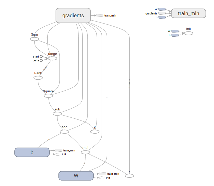
+ 이 코드의 함수를 시각화 해서 본다면
tf.contrib.learn
tf.contrib.learn은 다음을 포함하여 기계 학습의 메커니즘을 단순화하는 상위 TensorFlow 라이브러리입니다.
-실행중인 학습 루프
-평가 루프 실행
-데이터 세트 관리
-수유 관리
tf.contrib.learn은 많은 공통 모델을 정의합니다.
기본 사용법
tf.contrib.learn을 사용하면 선형 회귀 프로그램이 얼마나 단순 해지는 지 주목하십시오
import tensorflow as tf
# NumPy is often used to load, manipulate and preprocess data.
import numpy as np

# Declare list of features. We only have one real-valued feature. There are many
# other types of columns that are more complicated and useful.
features = [tf.contrib.layers.real_valued_column("x", dimension=1)]

# An estimator is the front end to invoke training (fitting) and evaluation
# (inference). There are many predefined types like linear regression,
# logistic regression, linear classification, logistic classification, and
# many neural network classifiers and regressors. The following code
# provides an estimator that does linear regression.
estimator = tf.contrib.learn.LinearRegressor(feature_columns=features)

# TensorFlow provides many helper methods to read and set up data sets.
# Here we use `numpy_input_fn`. We have to tell the function how many batches
# of data (num_epochs) we want and how big each batch should be.
x = np.array([1., 2., 3., 4.])
y = np.array([0., -1., -2., -3.])
input_fn = tf.contrib.learn.io.numpy_input_fn({"x":x}, y, batch_size=4,
                                              num_epochs=1000)

# We can invoke 1000 training steps by invoking the `fit` method and passing the
# training data set.
estimator.fit(input_fn=input_fn, steps=1000)

# Here we evaluate how well our model did. In a real example, we would want
# to use a separate validation and testing data set to avoid overfitting.
print(estimator.evaluate(input_fn=input_fn))
{'global_step': 1000, 'loss': 1.9650059e-11}+ 위 처럼 결과가 나올 것입니다.
커스텀 모델
tf.contrib.learn은 사용자를 미리 정의 된 모델로 잠그지 않습니다.
TensorFlow에 내장되어 있지 않은 커스텀 모델을 만들고 싶다고 가정 해 보겠습니다.
tf.contrib.learn의 데이터 세트, 수유, 교육 등의 높은 수준의 추상화는 여전히 유지할 수 있습니다.
설명을 위해, 우리는보다 낮은 수준의 TensorFlow API에 대한 지식을 사용하여 LinearRegressor에 대한 자체 등가 모델을 구현하는 방법을 보여줍니다.
tf.contrib.learn과 작동하는 사용자 정의 모델을 정의하려면 tf.contrib.learn.Estimator를 사용해야합니다. tf.contrib.learn.LinearRegressor는 실제로 tf.contrib.learn.Estimator의 하위 클래스입니다.
Estimator를 하위 분류하는 대신 Estimator에게 예측, 교육 단계 및 손실을 평가할 수있는 방법을
tf.contrib.learn에게 알려주는 model_fn 함수를 제공하기 만하면됩니다. 코드는 다음과 같습니다.
import numpy as np
import tensorflow as tf
# Declare list of features, we only have one real-valued feature
def model(features, labels, mode):
  # Build a linear model and predict values
  W = tf.get_variable("W", [1], dtype=tf.float64)
  b = tf.get_variable("b", [1], dtype=tf.float64)
  y = W*features['x'] + b
  # Loss sub-graph
  loss = tf.reduce_sum(tf.square(y - labels))
  # Training sub-graph
  global_step = tf.train.get_global_step()
  optimizer = tf.train.GradientDescentOptimizer(0.01)
  train = tf.group(optimizer.minimize(loss),
                   tf.assign_add(global_step, 1))
  # ModelFnOps connects subgraphs we built to the
  # appropriate functionality.
  return tf.contrib.learn.ModelFnOps(
      mode=mode, predictions=y,
      loss=loss,
      train_op=train)

estimator = tf.contrib.learn.Estimator(model_fn=model)
# define our data set
x = np.array([1., 2., 3., 4.])
y = np.array([0., -1., -2., -3.])
input_fn = tf.contrib.learn.io.numpy_input_fn({"x": x}, y, 4, num_epochs=1000)

# train
estimator.fit(input_fn=input_fn, steps=1000)
# evaluate our model
print(estimator.evaluate(input_fn=input_fn, steps=10))
커스텀 모델 () 함수의 내용이 저수준 API의 수동 모델 트레이닝 루프와 얼마나 흡사한지 주목하십시오.
다음 단계
이제 TensorFlow의 기본 지식을 습득했습니다. 우리는 더 많은 것을 배우기 위해 여러분이 볼 수있는 튜토리얼을 몇 가지 더 가지고 있습니다. 초보자의 경우 초보자 인 경우 MNIST를 참조하십시오. 그렇지 않은 경우 전문가를위한 Deep MNIST를 참조하십시오
+ 다음 튜토리얼은 손글씨 인식을 하는 것입니다.
+ 이번 튜토리얼에서는 API에서 얼만큼 잘 제공해주는지 알려주는 것 같았습니다.
+ 다음 튜토리얼 부터는 점점 머신러닝과 관련하여 인곤지능과 가까워질 것 입니다.
+ 다 같이 힘내봅시다.
'Computer_IT > tensorflow' 카테고리의 다른 글
| Deep MNIST for Experts ( 히든 레이어 버전) (0) | 2017.06.30 |
|---|---|
| [인공지능] Tensorflow 프로그래머 가이드부터 다시 시작하자. (0) | 2017.06.22 |
| [인공지능] 초급 손글씨 판별하기 (MNIST For ML Beginners) (0) | 2017.06.14 |
| [인공지능] TensorFlow 시작하기 (설치 이후 첫 튜토리얼) (0) | 2017.05.22 |
| 인공지능의 입문 Tensorflow를 설치해보자. (0) | 2017.05.04 |